Summary: ‘A Theoretical Framework for Inference Learning’

I am excited to announce the paper ‘A Theoretical Framework for Inference Learning’ was recently excepted to the NeurIPS 2022 conference. It was authored by me (Nick Alonso), Beren Millidge, Jeff Krichmar, and Emre Neftci. The paper develops a theoretical/mathematical foundation for the inference learning algorithm, the standard algorithm used to train predictive coding (PC) models of biological neural circuits. This theoretical foundation could provide a basis for a theory of how the brain solves the credit assignment problem (explained below), and as a basis for further developing the algorithm for engineering applications. Here, I provide a brief intuitive summary of the mathematical/theoretical results, related simulation results, and their potential significance for neuroscience and engineering. A draft of the paper can be found on arxiv (here).

Introduction

How can a neural network, with multiple hidden layers, be trained to minimize some global loss function (where the loss is a measure of network performance)? This question is, roughly, what some refer to as the credit assignment problem for deep neural networks, as it involves determining the amount and direction (positive or negative) that network parameters affect the loss (i.e., ‘assigning credit’ to the parameters for how they affect the loss).

At least two things are needed for a satisfying solution to the credit assignment problem: First, is, what I will call, an optimization method, which is a general strategy for updating model parameters (synaptic weights, in the case of neural networks), which has guarantees of minimizing the loss function and converging to a local minimum of the loss. The optimization strategy also typically has a simple (one equation) description of how the loss relates to parameter updates, and in so doing provides an assignment of credit. Second, is an algorithmic implementation of the optimization strategy, which is a set of equations and step by step procedure (i.e., a program) which is used to compute the parameter updates.

Within the field of deep learning, the standard solution uses stochastic gradient descent (SGD) as its optimization method and the error backpropagation algorithm (BP) as its algorithmic implementation. The BP-SGD strategy works amazingly well in practice, however there are two issues facing BP-SGD. The first is a problem for neuroscience the second for neuromorphic engineering. 1) It is generally agreed that the brain is likely not doing BP. More biologically plausible algorithmic implementations of SGD have been developed. However, they still have some properties difficult to reconcile with neurobiology (discussed more below). 2) BP is difficult to implement in energy efficient, neuromorphic hardware, for similar reasons as to why it is biologically implausible. These issues motivate the search for more bio-compatible learning algorithms.

The inference learning algorithm (IL), which used to train popular predictive coding (PC) models of the brain, is one promising candidate. In 2017, James Whittington and Rafael Bogacz (see here) developed two important results concerning predictive coding networks and the inference learning algorithm (IL). First, they showed PC models, which are a kind of recurrent neural network, and the IL algorithm, can be used to train deep neural networks. Subsequent work has further established this on other datasets and tasks. Second, IL parameter updates approach those produced by BP in a certain limit.

However, the limit where IL approaches BP is a limit that is never fully realized in practice and is poorly approximated early in training. This essentially implies IL never equals BP in practice. This leaves us with some questions: Is IL just a rough/approximate implementation of SGD? Or might IL be implementing some other optimization strategy? Also, since IL is not doing BP exactly, in what ways does it differ from BP?

Main Result: Part 1

These were the questions explored in our paper ‘A Theoretical Framework for Inference Learning’. Our main result is that, under certain assumptions well approximated in practice, IL implements an optimization strategy known as implicit stochastic gradient descent (implicit SGD). Importantly, implicit SGD is distinct from the standard SGD that BP implements. We call standard SGD explicit SGD, for reasons we now explain. Here’s is a general mathematical description of explicit and implicit SGD:

Explicit SGD:

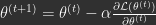
Implicit SGD:

Explicit SGD, which is implemented by BP, takes a gradient step over the parameters with some step size . This gradient can be readily and explicitly computed given the known values at the current training iteration, t. Hence, it is called explicit gradient descent. Implicit SGD, on the other hand, takes the gradient of the loss using the parameters at the next training iteration, t+1, and uses this gradient to update the parameters at the current training iteration, t. Generally, this gradient cannot be readily computed given known values at the current iteration t (e.g., the parameters at the next iteration are not known). However, it turns out the implicit SGD update is equivalent to the output of an optimization process known as the proximal operator, shown on the right hand side of the implicit SGD equation. The proximal operator sets the new parameters equal to the parameters that both minimize the loss, , and the norm of the change in parameters, i.e., it finds the parameters that best minimize the loss while remaining in the proximity of the current parameters. Hence, the implicit SGD update can be computed implicitly in terms of this optimization process/proximal operator.

(Note: those familiar with the explicit and implicit Euler methods from differential equations will notice that explicit and implicit gradient descent are analogous to these Euler methods.)

Main Results: Part 2

In what ways do explicit and implicit gradient descent (implemented via BP and IL respectively) behave differently? We studied this question in the paper through both theoretical results and simulations. Here’s a summary of the results:

First, IL is less sensitive to learning rate than BP. This is consistent with our theoretical interpretation, since is well known that explicit SGD is highly sensitive to learning rate, while implicit SGD is highly insensitive to learning rate. This insensitivity is due to the way the proximal operator uses the learning rate to only weight the two terms in the proximal objective function, rather than to scale the update, as explicit SGD does. Implicit SGD, in fact, has the property of unconditional stability, which means roughly that it will reduce the loss at the current iteration for essentially any positive learning rate.

Second, IL tends to take a more direct path toward local minima than BP, which is consistent with our theoretical interpretation. Explicit SGD follows the path of steepest descent each update. This implies, that if we imagine a non-convex (i.e., non-bowl shaped) loss landscape, explicit SGD will not take the most direct/shortest path toward local minima, but will often end up taking a longer, more round about way to find a minimum. This means parameters need to change more (i.e., long path length), in order to find a loss minimum. Implicit SGD, on the other hand, takes a shorter more direct path toward minima, since it aims to find the minimum norm (smallest parameter changes) needed to reduce loss significantly.

Third, shorter paths toward minima tend to mean quicker reduction of loss. We find this is especially true in the case of online learning where a single data-point is presented each iteration (see paper for a discussion of why this result may be more significant in online case).

Fourth, we find that IL updates tend to have a larger effect than BP on the input-output mapping of the network relative to their weight update magnitude. In this sense, IL updates are more impactful than BP updates. This is consistent with the implicit-SGD interpretation. The proximal operator can be interpreted as outputting the parameters that are most impactful, i.e., having largest impact on loss, and thus input-output mapping, relative to update magnitude.

Implications for Neuroscience

It is generally agreed BP is hard to reconcile with neurobiology (see [1], [2], [3] for good discussion). In response, some have developed alternatives to BP that exactly or approximately implement explicit SGD and better fit neurobiology. However, these more biologically inspired variants of BP still have some implausibilities. For example, in every BP alternative I have seen, feedback signals do not alter feedforward neuron activities (or if they do, performance worsens) (e.g., [4], [5]). This is difficult to reconcile with the fact that the brain is highly recurrently connected and local feedback and feedforward signals will essentially always interact with each other, either directly or indirectly through interneurons. IL, on the other hand, is implemented by predictive coding circuits, which are recurrent neural circuits where feedforward and feedback necessarily must interact (feedforward signals affect feedback signals and vice versa). Predictive coding circuits have also been mapped in highly detailed ways to cortical and subcortical circuits in the brain. There is still much debate about whether the brain is implementing PC widely, but it is clear the mechanics of IL avoid most of the biological implausibilities of BP and similar algorithms. This suggests a novel hypothesis concerning the optimization strategy used by the brain to solve the credit assignment problem: the brain solves the credit assignment problem through an implementation of implicit SGD, via an algorithm possibly similar to IL algorithm. The results above further characterize how learning in the brain should behave differently than BP/explicit SGD if this hypothesis were true, and thus suggests possible ways to test the two hypotheses.

Implications for Machine Learning

Neuromorphic hardware is computer hardware inspired by the brain. It typically uses spiking/binary networks, and is far more energy efficient than standard hardware. BP is hard to implement on neuromorphic hardware for several reasons. One of which is that BP uses weight updates that are not local in space and time. Like the brain, synaptic weight updates on neuromorphic hardware tend to require changes based on the activities of neurons at pre and post-synaptic layers (spatial locality) at a particular point in time (temporal locality). Exact BP requires storing feedforward activities through time and are thus not local in time, which cannot be done easily on neuromorphic hardware. IL, on the other hand, does not have to store neuron activities through time. It can essentially update synapses with whatever the pre and post-synaptic neuron activities are at just about any point in time during recurrent processing and still performs well. We did not implement a spiking version of IL, but if something akin to IL can be implemented in spiking networks, the weight updates it produces should be easier to implement on neuromorphic hardware.