Predictive Coding: A Brief Introduction and Review for Machine Learning Researchers

By Nick Alonso

Introduction

Predictive coding (PC), a popular neural network model used in neuroscience, has recently caught the attention of the machine learning community. A flurry of recent work has shown that PC and its synaptic update rules are to be able to train deep neural networks competitively with backpropagation (BP) and have interesting formal connections to backpropagation, expectation maximization, and other optimization methods. These results combined with the fact that PC uses local, biologically plausible learning rules makes PC of particular interest to the bio-inspired and neuromorphic computing communities. However, the recent literature on PC can be difficult to navigate for the machine learning researcher newly acquainted with PC, given the wide variety of names, terms, and variations that have emerged with this recent work. This brief review aims to 1) clarify the terminology around PC, 2) present a brief introduction to the PC approach to training deep networks, 3) review the recent theoretical work linking PC with various optimization methods and algorithms, and 4) discuss the pros and cons of PC compared to BP and future directions for its development.

This review will not discuss the neuroscience work behind PC. There already exist plenty of reviews on this subject. We provide a list of recommended classic papers and reviews below. For recent empirical work, we recommend Song et al. (2022) who discuss how the standard PC learning algorithm (called ‘inference learning’ below) differs from BP. They use this analysis to provide empirical support for the hypothesis that the brain learns in a way more similar to this standard PC algorithm than to BP.

Recommended Papers on Predictive Coding and the Free Energy Principle in Neuroscience

Rao, R. P., & Ballard, D. H. (1999). Predictive coding in the visual cortex: a functional interpretation of some extra-classical receptive-field effects. Nature neuroscience, 2(1), 79-87.

Friston, K. (2010). The free-energy principle: a unified brain theory?. Nature reviews neuroscience, 11(2), 127-138.

Bastos, A. M., Usrey, W. M., Adams, R. A., Mangun, G. R., Fries, P., & Friston, K. J. (2012). Canonical microcircuits for predictive coding. Neuron, 76(4), 695-711.

Keller, G. B., & Mrsic-Flogel, T. D. (2018). Predictive processing: a canonical cortical computation. Neuron, 100(2), 424-435.

Song, Y., Millidge, B. G., Salvatori, T., Lukasiewicz, T., Xu, Z., & Bogacz, R. (2022). Inferring Neural Activity Before Plasticity: A Foundation for Learning Beyond Backpropagation. bioRxiv.

Terminology

The term ‘predictive coding’ is sometimes used ambiguously machine learning literature. In what follows, it will be important to keep our definitions clear, so we first make a distinction between three components of a neural network: network architecture, learning algorithm, and optimization method. These concepts may seem straightforward to the machine learning researcher, but they are sometimes conflated in the PC literature.

Network Architecture: The set of equations defining how neuron states are computed and how neurons interact with each other via synaptic weights.
Optimization Method: A general technique for updating model parameters to minimize some loss function, e.g., stochastic gradient descent (SGD). Usually this technique describes in a simple way (one equation) how the loss relates to parameters updates.
Learning Algorithm: A step by step procedure for computing parameter updates, which ideally implements an optimization method with convergence guarantees (e.g., BP is an algorithm that implements SGD).

PC is sometimes referred to as an algorithm (e.g., ‘the predictive coding algorithm’) and other times referred to as an architecture (e.g., ‘predictive coding circuits’). Here we refer to PC as a kind of recurrent neural network architecture. Details of the PC architecture are described in the next section. Defining PC as an architecture allows us to distinguish between different learning algorithms that all utilize PC, and stays truer to the original neuroscience description of PC as a kind of circuit.

What Predictive Coding is and How it Works

Here we describe how PC works in standard multi-layered perceptron (MLP) architectures trained on supervised learning tasks, though it should be noted PC can also be used for self-supervised learning, as described below in the section on associative memory and self-supervised learning.

Consider a standard MLP architecture with neurons at layer $l$ represented as a column vector $h_l$ and weights $W_l$ that propagate signals from layer $l$ to $l+1$ . Neuron feedforward (FF) activities are computed $h_{l+1} = f(W_l h_l)$ , where f is a non-linearity. Note, when we use $h$ without a subscript, we refer to all neuron activities at all layers, and when we use $\theta$ we are referring to all parameters in the model. At each training iteration $t$ , input data $x^t$ and output prediction target $y^t$ are given to the network. (One can also think of these as mini-batches of data-points and targets, it does not change the algorithm described below). The network is tasked with minimizing some measure of loss, $\mathcal{L}(y^t, h_L^t)$ , where $h_L^t$ are the output layer FF activities.

There are several learning algorithms that use PC which are able to minimize the loss, $\mathcal{L}(y^t, h_L^t)$ , produced by the feedforward pass. Here we describe the standard learning algorithm that uses PC, sometimes referred to as inference learning (IL). IL can be described as a kind of energy-based algorithm that proceeds in two steps, both of which minimize a quantity known as free energy (F). We first describe the steps, then we describe the energy:

Inference Learning Algorithm (Informal)

(Inference Phase) Minimize/Reduce F w.r.t. neuron activities, while holding fixed weights.
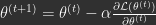
(Weight Update) Minimize/Reduce F w.r.t. synaptic weights, while holding fixed neuron activities.

We write ‘minimize/reduce’ because in practice F is typically not fully minimized in either step. The first step is sometimes called the inference phase, since it can be interpreted as performing approximate Bayesian inference. see section on expectation maximization for brief discussion of this interpretation. For details Bogacz (2017).

What is free energy? Since we are altering the feedforward activities in step 1, we need new notation to refer to altered\optimized activities. We will call the altered\optimized activities computed in step 1 as $\hat{h}$ . One description of free energy, used in Alonso (2022), applied to standard MLP architectures is

$F(\hat{h}, \theta) = \mathcal{L}(y^t, \hat{h}_{L}) + \sum_l^{L-1} \frac12 \Vert \hat{h}_{l+1} - f(W_l \hat{h}_l) \Vert^2 + \gamma^{decay} \sum_l^{L} \frac12 \Vert \hat{h}_l \Vert^2$ .

In words, free energy, F, is a positive scalar that depends on the loss between target activities $y^t$ and $\hat{h}_L$ , the difference between $\hat{h}_{l+1}$ and the previous layer’s output $f( W_l \hat{h}_l)$ , and the magnitude of the activities. (Note it is also possible to use $W_l f(\hat{h}_l)$ instead of $f(W_l \hat{h}_l)$ ).

It is common in practice to ‘fully clamp’ output layer activities such that $\hat{h}_L = y^t$ and $\mathcal{L}(y^t, \hat{h}_L^t) = 0$ and to ignore the decay term (set $\gamma^{decay}=0$ ). Further, it is standard to describe the outputs $f(W_l \hat{h}_l)$ as predictions of $\hat{h}_{l+1}$ . Let’s therefore define the prediction at layer $l+1$ as $p _{l+1} = f(W_l \hat{h}_l)$ . Under these conditions, F simplifies to

$F(\hat{h}, \theta) = \sum_{l=1}^{L} \frac12 \Vert \hat{h}_{l} - p_{l} \Vert^2 = \sum_{l=1}^{L} \Vert e_{l} \Vert^2$

In this case, F is just the summation over squared prediction errors, $e_l$ , at each layer $l$ . For a detailed probabilistic interpretation of F see Bogacz (2017).

A formal description of IL can now be expressed as follows:

Inference Learning Algorithm (Formal)

$\hat{h}^t \approx \text{argmin}_{\hat{h}} F(\hat{h}, \theta^t)$
$\theta^{t+1} \approx \text{argmin}_{\theta} F(\hat{h}^t, \theta)$

Where does PC fit into this algorithm?

PC refers to the process of iteratively updating neuron activities to reduce local squared prediction errors.

By ‘local’, we mean that neurons at layer $l$ are only updated to reduced the squared prediction errors at layer $l$ and $l+1$ . Typically, though not always, these updates are gradients of the local errors w.r.t. neuron activities and can be interpreted as recurrent neural network computations. Again, the term ‘predictive coding’ is used a bit loosely in the literature, but we think this captures what neuroscientists and much of the machine learning community working on these algorithms are referring to when they use the term ‘predictive coding’. Formally, here is how PC updates neuron activities using gradients of the local errors:

$\hat{h}_l = \hat{h}_l - \gamma \frac{\partial F}{\partial \hat{h}_l} = \hat{h}_l + \gamma (W_l^{\top}f'(W_l\hat{h}_l) e_{l+1} - e_{l})$ ,

where $\gamma$ is the step size and f’ is the gradient of the non-linearity. We emphasize that these are only partial gradients, since these updates only use gradients of errors at layers $l$ and $l+1$ , and ignore error gradients from other layers. We can see that this looks like a sort of recurrent neural network computation where predictions are propagated in one direction, then prediction errors are propagated back to the prediction generating neurons using the weight transpose. (This transpose may also be replaced with a separate matrix that learns to approximate the transpose).

In practice, each training iteration, neuron activities are updated with multiple gradient updates (typically about 10-25) so F is sufficiently reduced. Afterward, weights are usually updated with a partial gradient step over weights:

$W_l^{t+1} = W^{t} - \alpha \frac{\partial F}{\partial W_l} = W^{t} + \alpha e_{l+1}f'(W_l\hat{h}_l)\hat{h}_l^{\top}$ ,

where $\alpha$ is the step size. Again, these updates only use local error information: $W_l$ is updated with gradient of the squared error at layer $l+1$ . In the case where mini-batches are used, these updates are summed or averaged over the mini-batch. If we assume there exist error neurons encoding $e_{l+1}$ this update is a Hebbian-like learning rule that is the outer product of presynaptic activities $\hat{h}_l$ and post-synaptic error neuron activities, $e_{l+1}$ , with local modulation $f'(W_l\hat{h}_l)$ .

One last thing to note. When using gradient descent to update neuron activities, it seems necessary, in practice, to initialize activities to the FF activities. That is, initialize $\hat{h}$ to $h$ . Taking this into account, we can now describe how PC is used to train MLPs:

Inference Learning via Predictive Coding (IL-PC)

Initialize activities to feedforward activities, $\hat{h} = h$
Reduce F w.r.t. $\hat{h}$ using gradient descent/PC, while holding fixed $\theta$ .
Reduce F w.r.t. $\theta$ using a gradient step, while holding fixed $\hat{h}$ .

Those familiar with backpropagation (BP) will realize IL has some dissimilarities from BP. For example, unlike BP, IL does not store and use feed-forward activities, $h$ , to compute weight updates. This raises a question: why is IL-PC able to minimize the loss, which is computed using feed-foward activities, $\mathcal{L}(y^t, h_L^t)$ , given it does not use these activities to compute weight updates? One can get an intuition for how this works by looking at the figure below. We discuss this and related questions in more detail in the following sections.

Another Recommended Tutorial

Bogacz, R. (2017). A tutorial on the free-energy framework for modelling perception and learning. Journal of mathematical psychology, 76, 198-211.

Predictive Coding, Backprop, and Stochastic Gradient Descent

Whittington and Bogacz (2017) were the first to show that IL-PC could be used to train MLPs on classification tasks, which raises the question of why IL-PC is able to minimize a loss. Whittington and Bogacz (2017) provided some useful insight into this question by showing that IL-PC updates become increasingly similar to BP updates in the limit where altered/optimized activities approach FF activities, i.e., $\hat{h} \rightarrow h$ . This suggests IL-PC is able to reduce the loss because it is approximating BP and thus stochastic gradient descent (SGD). However, with a fully clamped output layer, as used by Whittington and Bogacz, this limit is only approximated late in training when the loss is small and activities only need to be altered slightly to reduce local errors. Early in training, however, when the loss is large, this approximation is worse. Yet IL-PC reduces the loss in a stable manner early in training, which raises the question of whether there is a better description of how IL-PC is reducing the loss. Indeed, recent theoretical works have emphasized the differences between IL-PC and BP/SGD, which we discuss more below (e.g., see Song et al. (2022), Millidge et al. (2022), and Alonso et al. (2022)).

A related line of research has looked to alter the IL-PC algorithm to better approximate BP. Song et al. (2020) presented the Z-IL algorithm, which is equivalent to BP. This equivalence is achieved by updating weights at a specific step during the inference phase using a specific step size. Z-IL was later shown by Salvatori et al. (2021) to also yield this equivalence in convolutional networks. Millidge et al. (2020) developed an algorithm called activation relaxation which very closely approximates BP. This algorithm stores initial FF activities at hidden layers so they could be used during weight updates. Millidge et al. (2022) later showed that softly clamping the output layer so activities are only slightly nudged from their initial activities yields a better approximation of BP than fully clamping. It should be emphasized that all of these algorithms use the same/similar PC procedure for updating neuron activities (same inference phase). The only differences are the rules for updating the weights. An interesting property of these algorithms is that they provide a way of performing SGD using local learning rules. However, these variants do not clearly improve performance over standard IL-PC. Further, some of these alterations may be seen as biologically implausible.

References and Other Recommended Papers on Relation between PC and BP

Whittington, J. C., & Bogacz, R. (2017). An approximation of the error backpropagation algorithm in a predictive coding network with local hebbian synaptic plasticity. Neural computation, 29(5), 1229-1262.

Whittington, J. C., & Bogacz, R. (2019). Theories of error back-propagation in the brain. Trends in cognitive sciences, 23(3), 235-250.

Song, Y., Lukasiewicz, T., Xu, Z., & Bogacz, R. (2020). Can the Brain Do Backpropagation?—Exact Implementation of Backpropagation in Predictive Coding Networks. Advances in neural information processing systems, 33, 22566-22579.

Millidge, B., Tschantz, A., Seth, A. K., & Buckley, C. L. (2020). Activation relaxation: A local dynamical approximation to backpropagation in the brain. arXiv preprint arXiv:2009.05359.

Salvatori, T., Song, Y., Lukasiewicz, T., Bogacz, R., & Xu, Z. (2021). Predictive coding can do exact backpropagation on convolutional and recurrent neural networks. arXiv preprint arXiv:2103.03725.

Millidge, B., Song, Y., Salvatori, T., Lukasiewicz, T., & Bogacz, R. (2022). Backpropagation at the Infinitesimal Inference Limit of Energy-Based Models: Unifying Predictive Coding, Equilibrium Propagation, and Contrastive Hebbian Learning. arXiv preprint arXiv:2206.02629.

Millidge, B., Salvatori, T., Song, Y., Bogacz, R., & Lukasiewicz, T. (2022). Predictive Coding: Towards a Future of Deep Learning beyond Backpropagation?. arXiv preprint arXiv:2202.09467.

Alonso, N., Millidge, B., Krichmar, J., & Neftci, E. (2022). A Theoretical Framework for Inference Learning. arXiv preprint arXiv:2206.00164.

Millidge, B., Song, Y., Salvatori, T., Lukasiewicz, T., & Bogacz, R. (2022). A Theoretical Framework for Inference and Learning in Predictive Coding Networks. arXiv preprint arXiv:2207.12316.

Song, Y., Millidge, B. G., Salvatori, T., Lukasiewicz, T., Xu, Z., & Bogacz, R. (2022). Inferring Neural Activity Before Plasticity: A Foundation for Learning Beyond Backpropagation. bioRxiv.

Predictive Coding and Expectation Maximization

Those familiar with expectation maximization (EM) may have noticed EM looks quite similar to IL. EM is a standard algorithm used train probabilistic generative models, which are composed of parameters $\theta$ and hidden variables $h$ . EM proceeds in two steps: first, the ‘E-step’ is performed, which computes the posterior of $P(h|x, \theta)$ , given the parameters and the data $x$ . Then the ‘M-step’ is performed, which updates $\theta$ holding fixed $h$ to maximize the joint probability $P(h, x| \theta)$ . This same procedure is equivalent to another two step algorithm, where one first minimizes a quantity known as variational free energy w.r.t. $h$ holding fixed $\theta$ , then minimizes the same quantity w.r.t. $\theta$ holding fixed $h$ (see Neal and Hinton, 1998).

The energy-based version of EM sounds just like IL-PC. This is interesting given that IL-PC was created by Rao and Ballard (1999) in a neuroscience context, where they did not derive IL-PC from EM and made no mention of EM in their original paper. The similarities between IL and EM have been pointed out before, e.g., see Millidge et al. (2021) and Marino (2022). However, it was only recently shown under what assumptions IL is equivalent to EM by Millidge et al. (2022). Activities are assumed to represent the mean of Delta distributions, which act as the sufficient statistics of the approximate posterior distribution. The posterior means are computed in the E-step using, what is called variational inference, which approximates the posterior using some optimization method to reduce free energy (for tutorial on variational inference see Blei et al (2017), and Bogacz (2017)). Synapses encode the parameters of the generative model. This interpretation offers an alternative to the BP interpretation as to why IL-PC is able to minimize a loss, since EM has guarantees to converge to a minimum (or saddle point) of the log-likelihood of the data (Dempster (1977), Neal and Hinton (1998)).

References and Other Recommended Papers on PC and EM

Dempster, A. P., Laird, N. M., & Rubin, D. B. (1977). Maximum likelihood from incomplete data via the EM algorithm. Journal of the Royal Statistical Society: Series B (Methodological), 39(1), 1-22.

Neal, R. M., & Hinton, G. E. (1998). A view of the EM algorithm that justifies incremental, sparse, and other variants. In Learning in graphical models (pp. 355-368). Springer, Dordrecht.

Blei, D. M., Kucukelbir, A., & McAuliffe, J. D. (2017). Variational inference: A review for statisticians. Journal of the American statistical Association, 112(518), 859-877.

Bogacz, R. (2017). A tutorial on the free-energy framework for modelling perception and learning. Journal of mathematical psychology, 76, 198-211.

Millidge, B., Seth, A., & Buckley, C. L. (2021). Predictive coding: a theoretical and experimental review. arXiv preprint arXiv:2107.12979.

Marino, J. (2022). Predictive coding, variational autoencoders, and biological connections. Neural Computation, 34(1), 1-44.

Millidge, B., Song, Y., Salvatori, T., Lukasiewicz, T., & Bogacz, R. (2022). A Theoretical Framework for Inference and Learning in Predictive Coding Networks. arXiv preprint arXiv:2207.12316.

Salvatori, T., Song, Y., Millidge, B., Xu, Z., Sha, L., Emde, C., … & Lukasiewicz, T. (2022). Incremental Predictive Coding: A Parallel and Fully Automatic Learning Algorithm. arXiv preprint arXiv:2212.00720.

Predictive Coding and Implicit Gradient Descent

The EM interpretation provides an algorithmic description of IL-PC that is distinct from the BP interpretation. However, the EM interpretation alone does not provide a concise\clear description of how parameters are moving through parameter space. For example, is the variant of EM that IL-PC implements just another way of implementing/approximating SGD? Or should we interpret the algorithm as implementing some other optimization method, i.e., is it using some other strategy to move parameters through parameter space to find local minima?

Some progress on this questions is made by Alonso et al. (2022), who showed the IL algorithm used in standard MLP architectures closely approximates an optimization method known as implicit stochastic gradient descent (implicit SGD). Importantly, implicit SGD is distinct from the standard SGD that BP implements. We call standard SGD explicit SGD, for reasons we now explain. Here’s is a general mathematical description of explicit and implicit SGD:

Explicit SGD: $\theta^{(t+1)} = \theta^{(t)} - \alpha \frac{\partial \mathcal{L}(\theta^{(t)})}{\partial \theta^{(t)}}$

Implicit SGD: $\theta^{(t+1)} = \theta^{(t)} - \alpha \frac{\partial \mathcal{L}(\theta^{(t+1)})}{\partial \theta^{(t+1)}} = argmin_{\theta} \mathcal{L}(\theta) + \frac{1}{2\alpha}\Vert \theta - \theta^{(t)} \Vert^2$

Explicit SGD takes a gradient step over the parameters with some step size $\alpha$ . This gradient can be explicitly computed given the known values at the current training iteration, t. Hence, explicit gradient descent. Implicit SGD, on the other hand, takes a gradient step on $\theta^t$ , where the gradient is computed using the parameters at the next training iteration, t+1. Generally, this gradient cannot be readily computed given known values at the current iteration t (e.g., $\theta^{t+1}$ not known). However, it turns out the implicit SGD update is equivalent to the output of an optimization process known as the proximal operator, shown on the right hand side of the implicit SGD equation. The proximal operator sets the new parameters equal to the parameters that both minimize the loss, $\mathcal{L}$ , and the norm of the change in parameters. It finds the parameters that best minimize the loss while remaining in the proximity of the current parameters. Therefore, the parameters updated with implicit SGD can be computed implicitly in terms of this optimization process/proximal operator.

How does IL approximate implicit SGD? Here’s the rough intuition: minimizing F w.r.t. activities means clamping the output layer, reducing $\Vert e \Vert^2$ , and reducing $\Vert \hat{h}\Vert^2$ (via the decay term). Fully or softly clamping the output layer activities and updating the weights to reduce local errors will yield a new input/output mapping that reduces the loss given the same input, which is shown intuitively in the figure above. Second, reducing $\Vert e \Vert^2$ and $\Vert \hat{h}\Vert^2$ reduces the magnitude of weight updates, since weight updates are the outer product of $e$ and $\hat{h}$ . Thus, minimizing F w.r.t. neuron activities can be seen as finding target activities that will both reduce $\mathcal{L}(y^t, h_L)$ and reduce $\Vert \theta - \theta^t \Vert^2$ , just like implicit SGD. Importantly, there are differences between explicit and implicit SGD. For example, they typically do not move parameters through parameter space along the same path, and implicit SGD is far less sensitive to learning rate than explicit SGD. For details see the paper and/or summary referenced below.

Reference

Alonso, N., Millidge, B., Krichmar, J., & Neftci, E. (2022). A Theoretical Framework for Inference Learning. arXiv preprint arXiv:2206.00164.

Alonso, N. (2022) Summary: ‘A Theoretical Framework for Inference Learning’. https://neuralnetnick.com/2022/12/19/summary-a-theoretical-framework-for-inference-learning

Predictive Coding, Self-supervised Learning, and Auto-associative Memory

So far we have considered standard MLP architectures that attempt to map input $x^{t}$ to target output $y^t$ . However, PC was originally used to model self-supervised learning in the brain. In these tasks, the model is provided with some datapoint $x^{t}$ , and, similar to a hierarchical autoencoder, must compute hidden representations $h_0, h_1,...,h_L$ that generate predictions/reconstructions of the data and other hidden representations. In probabilistic terms, we want to learn a generative model $P(x, h)$ , that we can sample from and use to perform inference. Unlike more standard achitectures for this task, like variational autoencoders, PC networks do not use an encoder that directly maps $x \rightarrow h$ . Instead PC networks compute $h$ using the the recurrent processing (i.e., gradient descent) described above, which minimizes local prediction errors throughout the network. Recent work has shown that PC models are able to learn effective generative models, that perform inference and produce samples similar, and sometimes slightly better, in quality than variational autoencoders trained with BP on natural images (e.g., Ororbia & Kifer, 2022, Ororbia & Mali, 2022).

Another sort of self-supervised task is the auto-associative memory task. For this task, a model is trained in a self-supervised manner to input, represent, and reconstruct input data. However, during test time, corrupted versions of the training data, $\widetilde{x}$ , are presented where noise is added to the data or certain elements of the data are removed/set to 0. The model must return the uncorrupted version of the data (i.e., denoise or fill in missing elements). That is, we want the model to be able to learn the mapping $\widetilde{x}^t \rightarrow h \rightarrow x^t$ . Salvatori et al. (2021) recently showed that PC networks trained with IL can perform auto-associative tasks and outperform other standard auto-associative models like modern Hopfield networks, and PC networks are able do so on high-dimensional image vectors.

References

Ororbia, A., & Kifer, D. (2022). The neural coding framework for learning generative models. Nature communications, 13(1), 1-14.

Ororbia, A., & Mali, A. (2022). Convolutional Neural Generative Coding: Scaling Predictive Coding to Natural Images. arXiv preprint arXiv:2211.12047.

Salvatori, T., Song, Y., Hong, Y., Sha, L., Frieder, S., Xu, Z., … & Lukasiewicz, T. (2021). Associative memories via predictive coding. Advances in Neural Information Processing Systems, 34, 3874-3886.

Pros and Cons of IL-PC and Future Directions

Why should a machine learning practitioner or researcher care about IL-PC and its variants? Here we list some advantages and disadvantages of IL-PC compared to BP and possible future research directions.

Advantages:

Unlike BP, weight updates performed by IL-PC are local in space and time: IL-PC uses update rules that are the product of presynaptic activities and post-synaptic error neuron activities. BP updates are not spatially local in this way, since error signals are propagated directly from the output layer. IL-PC updates are local in time since they use whatever activities and local errors are available at the time of the updates, whereas BP must store FF activities during the forward and backward pass through time. The locality of its updates suggests IL-PC may be more compatible with neuromorphic hardware than BP. However, it is not obvious how to convert the IL-PC algorithm here to spiking networks, which are often required on neuromorphic hardware, e.g., do we need to encode errors in spiking neurons? If so how? How should gradient updates on activities work given spikes are not differentiable? These questions are not necessarily problems, but they will require engineering work to solve.
Work by Song et al. (2022), Alonso et al. (2022), and Salvatori (2021) suggest possible performance advantages of IL-PC over BP. For example, some improved performance, either in terms of training speed or loss at convergence, were observed under data constraints, small mini-batches, concept drift, and auto-association with large images. However, the extent of these advantages needs to be further explored and better established.

Disadvantages:

The inference phase of the IL-PC algorithm is computationally expensive, since activities must be updated multiple times each training iteration. Future work could look to reduce the computational cost of this phase by altering the algorithm in various ways. The computational cost could possibly also be reduced with highly correlated data (e.g., video), since the network activities may not need to be reset and recomputed each iteration. This would need to be tested, however.
IL-PC is trickier to implement than BP: there are standard libraries for automatically computing gradients, while PC-IL must be implemented by hand. Future work could attempt to find efficient implementations of PC-IL written in an open source library that can perform IL-PC ‘under the hood’ for arbitrary architectures.

Finally, we also believe that there is much potential to further explore IL-PC for self-supervised tasks. IL-PC, which as noted above is a special case of EM, is most useful for models where probabilistic inference is part of the task being performed, since an inference step (or E-step) is ‘built into’ the algorithm. When this inference phase is not used to perform the task, the inference phase/E-step adds significantly to the computational cost while only providing learning signals. The classification tasks considered above, for example, do not use the inference phase during test time to predict labels. It is only used during training to provide learning signals. Salvatori et al.’s and Orobia et al.’s work on auto-associative memory and self-supervised learning are good examples of a self-supervised task where the inference phase of IL-PC actually performs the task (i.e., the inference phase did the reconstruction, denoising, and filling-in of the input image). Applying IL-PC to self-supervised learning tasks also utilizes the algorithm for what it was originally designed for: brain-like self-supervised learning.